In the long (context) run
It’s not the quadratic attention; it’s the lack of long pre-training data
One intriguing trend in the field of Large Language Models (LLMs) is the growing context length — the numbers of tokens we can feed to the Transformer before it predicts the next tokens. Especially in the past year we’ve seen a remarkable push towards long-context LLMs, see the Figure below.
A significant turning point was the invention of FlashAttention, a clever way to lay out the attention computation on modern GPUs, leading to improved computational and memory efficiency. While we won’t go into the technical details, this technique removed a GPU memory bottleneck and enabled LLM developers to increase the context length from the conventional 2K tokens to the 8-65K range.
Interestingly, if you look a bit closer at the long-context LLMs you’ll see that many of them are finetuned versions of base LLMs with much smaller context windows. For example:
- Yarn-Llama-2-7B-128k (128K context) is fine-tuned from Llama-2-7B (4K context)
- Code Llama (16K context) was fine-tuned from a 4K base model
- MPT-7B-StoryWriter (65K context) is finetuned from MPT-7B (2K context)
- GPT-4 supposedly underwent a two stage training process with a 8K base training and a 32K finetuning stage.
Why do we have these two training phases? Is it (1) computationally too expensive to train with long contexts because of the quadratic complexity of the attention layer or (2) is it the lack of long sequence data in the pre-training phase?
In this post, we’re going to dive into both aspects:
- What’s the computational overhead of the attention layer as we increase the context length? We’ll derive the training FLOPs of the Transformer model and investigate the overhead of the quadratic attention operator. We’ll find that the overhead depends on the hidden state dimension and that context windows of 16-32K are manageable for current model scales.
- We’ll investigate the distribution of sequence lengths in common pre-training datasets, such as Github and CommonCrawl. Interestingly, we’ll see that over ~80% of pre-training examples, whether they are web documents or code files, consist of fewer than 2K tokens. On the other hand, we observe that a few lengthy files disproportionally impact the token count (especially for source code), with over 30-50% of the tokens coming from files with over 8K tokens.
Taking these observations together, it suggest that while pre-training with 16-32K context window is feasible, the token distribution of individual documents is not well-suited for it. The main issue is that the conventional pre-training approach packs tokens from random files into the context window. This would lead to many unrelated documents within a 16-32k token window. Assuming that LLMs benefit from more meaningful long-context during pre-training, one idea I’d like to put forward with this post is to leverage the meta-data to create longer pre-training data, e.g. by connecting web documents through hyperlinks and linking code files through repository structure.
1. The impact of context length on Transformer FLOPs
Let’s start our exploration by investigating the computational overhead of the attention layer. We are going to estimate the compute needed for training the Transformer model. More specifically, we are calculating the floating point operations (FLOPs) of the matrix multiplications in the model during the forward and backward pass. For our investigation, we split the FLOPs into three groups: the dense layers in the feedforward layer (FFN), the query, key, value, and output projections (QKVO), and calculating the query-key scores and the weighted sum over the value embeddings (Att).
For a model with $N_l$ transformer layers, a hidden state dimension $d$, and context length $L$, the FLOPs per token (FLOPs/token) breakdown as follows: $$ \begin{align} &\text{FLOP}_{FFN} &=&~~~~ N_l (48 d^2)\\\ &\text{FLOP}_{QKVO} &=&~~~~N_l(24 d^2)\\\ &\text{FLOP}_{Att} &=&~~~~N_l (6d(L+1))\\\ \end{align} $$ See the Appendix for the derivation. It’s worth stressing that we look at FLOPs/token in order to meaningfully compare across different context lengths. Also note that $\text{FLOP}_{Att}$ is the only term depending on the context length $L$.
Now let’s investigate how much the three terms contribute to the total FLOPs/token as you increase the context length. Below, we show the breakdown for the LLaMA-7B model, with $\small d=4096$ and $\small N_l=32$). On top of each bar we display the relative contribution of the attention FLOPs: $\small \frac{\text{FLOP}_{att}}{\text{FLOP}_{FFN} + \text{FLOP}_{QKVO}}.$
As you can see, the contribution of the attention FLOPs is relatively small (8%) for a 4K context window. This is the pre-training regime for Llama-2 and several other base LLMs, where the attention FLOPs have a negligible impact on the computation. However, when utilizing a much larger context window of 128K (like Yarn-Llama-2), the attention FLOPs become the dominating factor, leading to a significant 260% overhead.
In practice this means that if a full pre-training run takes 1 week with a 2K context window, it is expected to take 3.5 weeks with a 128K context length. Of course, this assumes that training would involve the same number of tokens (e.g. by decreasing the batch-size). Given this substantial increase in compute time, many researchers and developers would only want to train with such overhead during the fine-tuning stage.
Between these two extremes there exists a compelling middle ground. For instance, employing an 8-16K context window leads to a manageable 16-33% overhead. This is the trade-off we chose for StarCoder, which was pre-trained with an 8K context length for over 1 trillion tokens.
What many people tend to underestimate is how the attention overhead is affected by the model size. Both the FFN FLOPs and QKVO FLOPs (as well as the model parameters!) grow quadratically with the hidden state dimension $d$. In the case of LLaMA-65B ($\small N_l=80$), the dimension $d=8192$ is twice the size of LLaMA-7B; This means we can double the context length while incurring the same overhead! In other words, using a 16-32K context window now results in the same 16-33% overhead.
For even bigger models like GPT3-170B ($\small d=12288, N_l=96$), it is possible to increase the context window to 64K with almost the same overhead (40%). Although it is unclear if we need such big models, see my previous post.
All in all, I’d say that training base models in the 16-32K range is very reasonable for current model scales. As I explain in the next section, the main bottleneck is that the datasets are not well-suited for pre-training with such long-context.
2. The sequence length of pre-training data
Now let’s investigate the distribution of sequence lengths in common pre-training datasets. Let’s start by examining LLaMA’s training data in the table below.
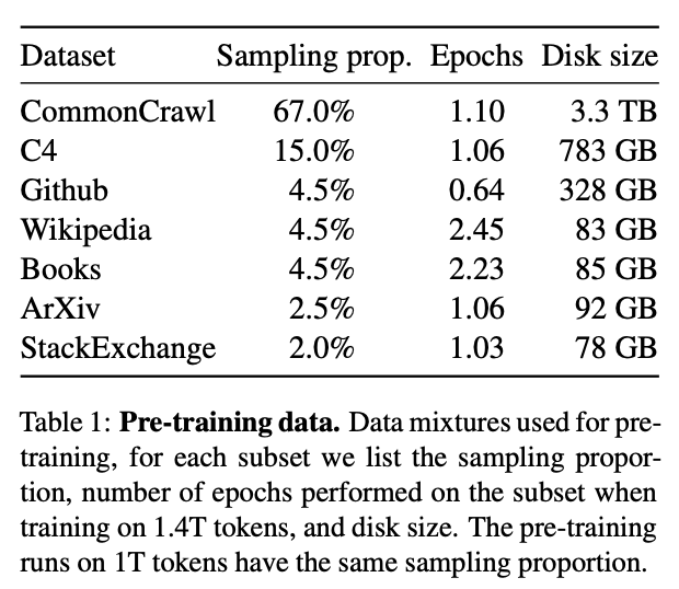 We see that the main data source is CommonCrawl — a publicly available crawl of the internet. In fact, C4 is also derived from CommonCrawl so this data source makes up over 80% of LLaMA’s training data. The other data sources—Github, ArXiv, Wikipedia, and books—contribute only a small fraction to the training data. Note that MPT-30B and OpenLLaMA-7B largely followed the same data distribution and Falcon-40B even trained exclusively on CommonCrawl data (see the RefinedWeb dataset).
In contrast, LLMs for code are usually trained on source code from Github. StarCoder, Replit-3B, CodeGen2.5, and StableCode all used The Stack, a pre-training dataset consisting of permissively licensed repositories from Github.
We are going to analyze the distribution of sequence lengths of these pre-training datasets. The main focus is on CommonCrawl and Github but we will also include smaller datasets like Wikipedia and Gutenberg books for reference. For each source, we’ll sample 10K examples, tokenize the samples, and save the sequence length. Subsequently, we will create histograms to visualize the sequence length distribution, examining how many documents or files fall into each bin (i.e., document count). Additionally, we’ll assess the token count within each bin, as we noticed that a few lengthy files can disproportionately impact the statistics. Note that we use the Falcon tokenizer for text-only sources (CommonCrawl, Wikipedia, Gutenberg) and the StarCoder tokenizer for source code (The Stack).
2.1 CommonCrawl
Let’s start with CommonCrawl and look at the RefinedWeb and C4 datasets. From the plot we immediately see that a significant portion of files in both C4 and RefinedWeb are relatively short, with over ~95% of them containing fewer than 2K tokens. Extending the context window beyond 2K will therefore capture longer context for only 5% of the files!
However, you might argue that we care about the number of tokens in each bucket rather than the number of documents. Indeed, the picture is slightly different when we look at the token count in the plot below. Almost 45% of the tokens in RefinedWeb are derived from files exceeding 2K tokens. Thus, increasing the context length beyond 2K might still be helpful for 45% of the tokens. For the remaining 55%, we would concatenate tokens from random files into the context window. I’d say that this is unlikely to benefit the model and might even hurt performance.
If we were to extend the context window to 8K, we would be able to fit the entire file within the context for almost 80% of the tokens. Or conversely, only 20% of the tokens would potentially benefit from a longer context than 8K.
Another noticeable discrepancy emerges from this plot—RefinedWeb exhibits a much longer tail than C4. We see that over 12.5% of the tokens in RefinedWeb are from files exceeding 16K tokens, while it is not even 2.5% for C4. It’s interesting that, despite both datasets originating from the same source, there’s such a significant difference in the sequence length distribution.
2.2 Github
Next, let’s look at different programming languages, Github issues, and Jupyter notebooks in starcoderdata — a subset of The Stack that was used for training StarCoder. For all programming languages, we again observe that the majority of files are short: over 80% have fewer than 3K tokens. Similarly, Github issues tend to be relatively short. We only observe slightly longer context in Jupyter notebooks, although over 80% of the files are still shorter than 5K tokens.
The document histogram also reveals there are more long files on Github than in CommonCrawl. This long-tail effect is more pronounced when we examine the token histogram below. Specifically, in case of the C programming language, we see that over 50% of the tokens originate from files exceeding 16K tokens - even though they account for less than 5% of the files! Upon manual inspections of these long files, I found that some exceed 300K tokens. Many of these lengthy files appeared to be large collections of macros and functions. Of course, you might question how much meaningful long-context structure you will find in such files.
Taking a broader perspective and considering other programming languages, it becomes clear that there are more lengthy code files than web documents. Excluding C and Javascript, we observe that approximately 50-70% of the tokens come from files with fewer than 8,000 tokens, whereas for RefinedWeb, this percentage was closer to 80%.
2.3 Other sources
As expected, we can find more long documents in other pre-training data sources, such as Wikipedia and books. In the histogram below, we observe that more than 50% of Wikipedia articles consist of over 4,000 tokens. In the case of books, such as the Gutenberg collection included in the LLaMA dataset, we even find that over 75% of these books contain more than 16,000 tokens.
Although this plot confirms these data sources possess more long-context structure than CommonCrawl and Github, they typically make up a relatively small portion of the training data. One contributing factor is that Wikipedia, for instance, is relatively small for large-scale pre-training, as it only consists of approximately 80GB of data, whereas CommonCrawl offers terabytes of data. On the other hand, books may not provide the comprehensive coverage of web documents and, therefore, typically represent a small percentage of the training data (4.5% for LLaMA, 3% for MBT-30B).
3. Discussion
3.1 Are we wasting attention overhead on randomly concatenated files?
We’ve seen that CommonCrawl and Github are the main data sources for training state-of-the-art open-source LLMs, and noticed that a substantial portion (about 80-90%) of its examples are shorter than 2K tokens. During pre-training we usually pack random examples into a single sequence until we’ve reached the maximum context length. With a 16-32K context length, this means we would spend much of the compute overhead on tokens that do not require communication between them. Besides wasting compute resources, this might also hurt performance as the model will be trained to ignore other tokens within the sequence.
3.2 How to obtain meaningful long-context data?
To begin with, it’s unclear what qualifies as “meaningful” long-context data. On the one hand, combining random files will certainly lack coherent connections between tokens in different files. On the other hand, tokens within a single file do not necessarily possess meaningful long-context structure. For example, upon closer examination of RefinedWeb and The Stack, I found that many long files appeared to be random collections of functions or text blocks. Moreover, in case of books or articles, you could argue that predicting the next token usually depends on local context, except perhaps for summaries and conclusions.
That being said, I do think it’s worth exploring how to better leverage a large context-window during pre-training. Given the longer-context data in Wikipedia and books, one obvious avenue is to seek out additional high-quality data sources, e.g., by obtaining licenses of textbooks or tutorials from publishers. Another promising direction is to move beyond concatenating random files into the context window and leverage the meta-data to curate more meaningful and coherent long-context data. Some ideas worth exploring:
- We can use hyperlinks between web documents. For example, LinkBERT proposes to put (passages of) linked documents in the same context and predict the relation between documents: continuation, random, or linked. This idea could be extended to decoder models by introducing special tokens for such predictions.
- We can use repository metadata to link files within the same code base. We could, with some probability, concatenate files from the same repository into the context window and create a similar linking objective by appending the repository name to the file content. Alternatively, we can identify heuristics to organize files within a particular repository, such as placing readme files at the end, with the goal of predicting repository descriptions based on a compilation of code files.
- We can use meta-information related to the evolution of source code files. Starcoderdata already includes single-file commits but this idea can be expanded by including commits over multiple files. We can also investigate including subsequent commits into the same context window. Similarly, we can leverage the edit history of text documents to create longer-context pre-training data.
3.3 Training with variable sequence length?
It is possible that we’ll have to accept the natural token distribution of text and source code and consider that creating longer-context pre-training data may not be helpful. While the current strategy is to split the training phase into a short-sequence pre-training phase followed by a long-sequence fine-tuning phase, it might be beneficial to pre-train directly with various sequence lengths. That is, instead of having a single pre-defined sequence length, we would divide the pre-training data into different buckets (e.g. <2K, <16K, <64K) and adjust the context length per batch (or every X batches). In this way, you would only pay the price of the attention overhead on files for long files.
3.4 How to evaluate long-context capabilities?
While I’m speculating that pre-training with a 16-32K context-window leads to more powerful base LLM, it’s important to acknowledge that the community still lacks robust benchmarks for evaluating long-context capabilities. In the absence of well-established benchmarks, we won’t be able to assess whether new long-context LLMs are effective or not. In the meantime, as we’ve seen in the CodeLLaMA paper, researchers resort to proxy tasks such as measuring the perplexity on long code files or the performance on synthetic in-context retrieval tasks. It’s an open question to what extend such evaluations transfer to real-world use cases such as repository-level code completion and question-answering/summarization for long financial reports or legal contracts.
I’m confident that the research community will tackle this evaluation issue over time. It remains to be seen whether my proposals for extending the context length are useful, but I hope my analysis have helped you better understand the trade-offs between context length, compute overhead, and (pre-)training data.
4. Limitations
- We only analyze the model FLOPs and abstract away the details of high performance computing, assuming that model training is compute-bound and achieves high GPU utilization for all model configurations.
- We do not consider how the context length impacts training dynamics. It is possible that training with long-context is less data efficient.
- Although my prediction is that in the short-to-medium term the quadratic attention operator is not the limiting factor, I do find the work on sub-quadratic attention models (Hyena, RWKV, etc) quite exciting, especially for domains outside of NLP (such as biology).
Acknowledgement
Thanks to Dzmitry Bahdanau, Oleh Shliazhko, Joel Lamy-Poirier, Leandro von Werra, and Laurent Dinh for helpful feedback on this post!
Appendix
Surprisingly, I couldn’t find a good derivation of the Transformer FLOPs that would support the above analysis. I’m adding such a derivation here to make this post more self-contained.
The Transformer
Before we start counting FLOPs, we need to define the operations in the Transformer model. Here, we focus solely on the Transformer layer and exclude the token embeddings, positional encodings, and output layer since, for large models, their impact is minor. Hence, we start from the embeddings $X^{0} \in \mathbb{R}^{bs\times L \times d}$ which are subsequently passed through $J$ transformer layers — see the definitions below. Note that many operations are batch matrix multiplications in which the weight matrix is broadcasted across the first dimension ($bs$).
$ \begin{align} &\mathbf{TransformerLayer}(X^{n} \in \mathbb{R}^{bs\times L \times d}): \\\ & (1)~~X^{n}_h = X^{n} + \text{MultiHeadAttention}(X^{n}) \\\ & (2)~~X^{n+1} = X^{n}_h + \text{FFN}(X^{n}_h) \\\ & \text{return}~X^{n+1} \\\ \end{align} $
$ \begin{align} & \mathbf{FFN}(X \in \mathbb{R}^{bs\times L \times d}): \\\ & (3)~~ H_{pre} = X \cdot W_{ffn1} \in \mathbb{R}^{bs\times L \times 4d} \\\ & (4)~~ H_{post} = \text{GeLU}(H_{pre}) \in \mathbb{R}^{bs\times L \times 4d} \\\ & (5)~~ Y \in \mathbb{R}^{bs\times L \times d} = H_{post} \cdot W_{ffn2} \\\ & \text{return}~Y \\\ \end{align} $
$ \begin{aligned} & \mathbf{MultiHeadAttention}(X \in \mathbb{R}^{bs\times L \times d}): \\\ & (6)~~ Q = X \cdot W_q \in \mathbb{R}^{bs\times L \times d} \\\ & (7)~~ K = X \cdot W_k \in \mathbb{R}^{bs\times L \times d} \\\ & (8)~~ V = X \cdot W_v \in \mathbb{R}^{bs\times L \times d} \\\ & (9)~~ O = [\text{head}_1; …; \text{head}_j; …; \text{head}_h] \cdot W_o \in \mathbb{R}^{bs\times L \times d} \\\ & \text{head}_j = \text{SelfAttention}(Q\tiny{[:, :, (j-1)*dh: j* dh]}, \normalsize{K}\tiny{[:, :, (j-1)*dh: j* dh]},\normalsize{V}\tiny{[:, :, (j-1)*dh: j* dh]}\normalsize) \in \mathbb{R}^{bs\times L \times dh} \\\ & \text{return}~O \\\ \end{aligned} $
$ \begin{aligned} & \mathbf{SelfAttention}(Q \in \mathbb{R}^{bs\times L \times dh}, K \in \mathbb{R}^{bs\times L \times dh}, V \in \mathbb{R}^{bs\times L \times dh}): \\\ & (10)~~ S = Q \cdot K^T \in \mathbb{R}^{bs\times L \times L} \\\ & (11)~~ P = \text{Softmax}(\frac{mask(S)}{\sqrt{dh}}) \in \mathbb{R}^{bs\times L \times L} \\\ & (12)~~ O = P \cdot V \in \mathbb{R}^{bs\times L \times dh} \\\ & \text{return}~O \end{aligned} $
Please find a summary and description of all the hyperparameters below.
| Parameter | Description |
|---|---|
| bs | batch size |
| d | the model size / hidden state dimension / positional encoding size |
| h | number of attention heads |
| dh | head dimension, usually $d/h$ |
| L | sequence length |
| $N_l$ | number of transformer layers |
| $X^{n} \in \mathbb{R}^{bs\times L\times d}$ | hidden state of $n^{th}$ layer |
| $W^{n}_{ffn1} \in \mathbb{R}^{d\times 4d}$ | Weight matrix of first feed-forward layer |
| $W^{n}_{ffn2} \in \mathbb{R}^{4d\times d}$ | Weight matrix of second feed-forward layer |
| $W^{n}_q \in \mathbb{R}^{d\times d}$ | Weight matrix of query projection |
| $W^{n}_k \in \mathbb{R}^{d\times d}$ | Weight matrix of key projection |
| $W^{n}_v \in \mathbb{R}^{d\times d}$ | Weight matrix of value projection |
| $W^{n}_o \in \mathbb{R}^{d\times d}$ | Weight matrix of output projection |
MatMul FLOPs
An important piece of background information is to understand how many floating point operations (FLOPs) are needed to perform a forward and backward pass through the model. Here, we specify this for the most FLOP-heavy operation: the matrix multiplication.
- Let’s consider the matrix multiplication $C = A \cdot B \in \mathbb{R}^{M \times N}$ where we have input matrices $A \in \mathbb{R}^{M \times K}$ and $B \in \mathbb{R}^{K \times N}$. The resulting matrix $C$ contains $M \times N$ elements, each obtained by obtained by doing a dot-product of K elements. Thus, we need $M \cdot N \cdot K$ operations to compute the matrix multiplications. Each operation involves a multiplication and addition so the total number of FLOPs is $2 \cdot M \cdot N \cdot K$. See this documentation from Nvidia.
- During the backward pass, we need to calculate the gradients $dA$ and $dB$. From the CS231n lecture notes, we know these are given by:
- $dA = dC \cdot B^T$. Because $dC \in \mathbb{R}^{M \times N}$ and $B^T \in \mathbb{R}^{N \times K}$, we have $2M\cdot K \cdot N$ FLOPs.
- $dB = A^T \cdot dC$. Because $A^T \in \mathbb{R}^{K \times M}$ and $dC \in \mathbb{R}^{M \times N}$, we have $2K\cdot N \cdot M$ FLOPs.
- In total we have $4MNK$, twice the number of FLOPs of the forward pass!
The Transformer FLOPs
Now let’s analyze how many FLOPs we need for the different parts of the Transformer layer. We will only look at the matrix multiplications and exclude element-wise operations such as layer normalization, GeLU activations, and residual connections. We also do not take into account the FLOPs needed to perform the optimization step.
FFN FLOPs
- For the linear projection in (1), we have $bs$ times $2 \cdot L \cdot 4d \cdot d$.
- For the linear projection in (3), we have $bs$ times $2 \cdot L \cdot d \cdot 4d$.
- In total, we have $16 bs L d^2$ for the forward pass and therefore $32 bs L d^2$ for the backward pass.
QKVO FLOPs
- To compute the query (6), key (7), value (8), and output embeddings (9), we need $2\cdot bs \cdot L \cdot d \cdot d$ FLOPS for each projection.
- In total, we have $8 bs L d^2$ for the forward pass, and $16 bs L d^2$ for the backward pass.
ATT FLOPs
- To calculate the attention scores (10), we need $2 bs\cdot L\cdot L \cdot dh$ FLOPs.
- To calculate the attention output (12), we need $2 bs\cdot L\cdot dh \cdot L$ FLOPs.
- We need to compute these two calculations for $h$ attention heads. Because $dh\cdot h = d$, the total FLOPs simplify to $4bsL^2 d$ for the forward pass. The backward pass requires $8bsL^2d$.
FLOPs per token
- If you increase the context length $L$, you also increase the number of the tokens we process in each model pass. In order to meaningfully compare the FLOPs for different context lengths, we will look at the FLOPs spend per token. In other words, we divide the total FLOPs in the previous paragraphs by $bs\cdot L$. Moreover, we’ve calculated the FLOPs for a single transformer layer and still need to multiply by $N_l$ to obtain the total FLOPs. This results in the following three terms: $$ \begin{align} &\text{FLOP}_{FFN} &=&~~~~N_l (48 d^2)\\\ &\text{FLOP}_{QKVO} &=&~~~~N_l (24 d^2)\\\ &\text{FLOP}_{Att*} &=&~~~~N_l(12 Ld)\\\ \end{align} $$ As we’ll show in the next paragraph, this actually overestimates the attention FLOPS because we do not take into account the autoregressive property of language models.
Overestimation of attention FLOPs
- Note that for autoregressive decoder models, tokens only attend to previous tokens in the sequence. This means that attention score matrix $S$ is a lower tridiagonal matrix and, as such, the upper diagonal doesn’t need to be calculated. As a result, the calculations in eq. 10 only require $bs\cdot (L+1) \cdot L \cdot dh$ FLOPs. Similarly, in the attention output calculations (eq. 12), the matrix $P$ is lower tridiagonal and therefore the FLOPs reduce to $bs\cdot (L+1) \cdot L \cdot dh$. The total attention FLOPs/token are therefore: $$ \begin{align} &\text{FLOP}_{Att} &=&~~~~N_l(6d (L+1))\\\ \end{align} $$
Relation to 6ND FLOP approximation
- It’s trivial to see how we get to the $6 N D$ formula for approximating the Transformer training FLOPs. First, note that the number of parameters for a transformer layer is given by $12d^2$. The total number of parameters $N$ are therefore related to the FLOPs/token as follows: $$6N = \text{FLOP}_{FFN} + \text{FLOP}_{QKVO}.$$ The number of training tokens $D$ is given by $bs \cdot L \cdot \text{num_train_steps}$. It’s worth noting that this approximation ignores $\text{FLOP}_{Att}$. As we’ve seen, this term is small for 2K context window but starts to dominate for longer context windows.